Fitting ELISA Data with R
Using R to fit your ELISAs might be slower and more fiddly than using [insert expensive software here] but sometimes the open source approach is much more satisfying - assuming you already know the basics.
Preparing the data
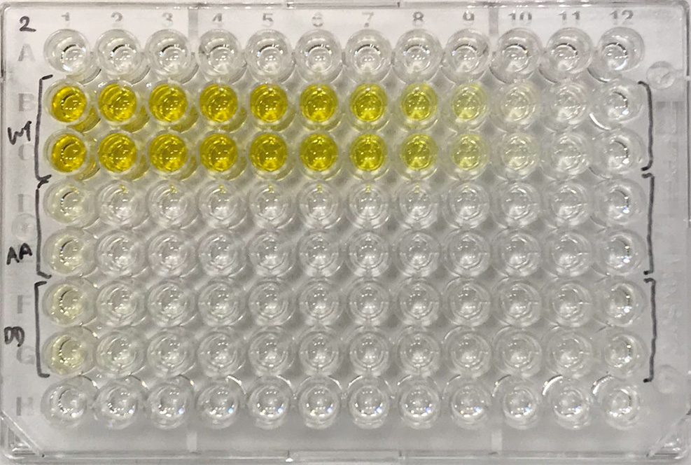
First we need to get the data into R. There are plently of ways you can do this but for now we’ll just enter some fictional readings manually and generate a range of 1⁄3 serial dilutions starting at 3 µM.
measurements   <- c(0.10, 0.15, 0.30, 0.68, 1.58, 3.08, 3.95, 3.97, 3.96)

serialdilute   <- function(x, n) {
  rev(x / 3^(1:n))
}

concentrations <- serialdilute(9e-6,09)

data <- data.frame(concentrations, measurements)
Now we have a data frame consisting of two columns: concentrations and measurements. Note: if you have repeat measurements (which you should), simply add further rows to the data frame with repeated concentrations and the new measurements.
concentrations measurements
1   4.572474e-10         0.08
2   1.371742e-09         0.09
3   4.115226e-09         0.10
4   1.234568e-08         0.15
5   3.703704e-08         0.30
6   1.111111e-07         0.68
7   3.333333e-07         1.58
8   1.000000e-06         3.08
9   3.000000e-06         3.95
If we plot those points with a log scale on the x axis then we should see our typical binding curve.
library(ggplot2)

ggplot(data = data) +
  geom_point( aes(concentrations,
                  measurements )) +
  scale_x_log10()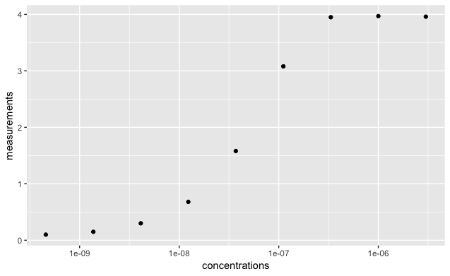
Fitting a model
To fit a nice curve to the data we need a model, in this case we can use a 4-parameter logistic model. In R we can fit our model using the Nonlinear Least Squares (nls) function. Specify some starting values which you can estimate from the first plot or autogenerate them (not discussed here) and run the function. Use the correlation (cor) function as a quick sanity check.
model4pl <- function(Concentration, Background, Mid, Slope, Bmax) {

  Bmax + ((Background - Bmax) / (1 + ((Concentration/Mid)^Slope)))

}


fit <- nls(measurements ~ model4pl(concentrations, Background, Mid, Slope, Bmax),
      data = data,
      start = c(Background=0, Mid=1e-7, Slope=1, Bmax=4),
      control = nls.control(maxiter=1000, warnOnly=TRUE) )

fit
# Nonlinear regression model
#  model: measurements ~ model4pl(concentrations, Background, Kd, Slope,     Bmax)
#   data: data
# Background        Mid      Slope       Bmax
# 1.619e-01  5.159e-08  1.470e+00  4.047e+00
# residual sum-of-squares: 0.0461
# Number of iterations to convergence: 7
# Achieved convergence tolerance: 3.636e-06

cor(data$measurements, predict(fit))
# [1] 0.9990598
In some cases you might get the following error message after running the nls. This means the model can’t converge, usually because the starting values were too far from the actual values. There are ways around this using so-called self-starting functions but by far the quickest method in my hands is to just make another an informed guess based on the first plot.
Warning message:
In nls(measurements ~ model4pl(concentrations, Background, Mid, Slope,  :
  singular gradient
When you’re happy that the model has converged, you can plot the fitted line by specifying the returned values to stat_function in ggplot.
ggplot(data = data) +
  geom_point(aes(concentrations, measurements))+
  scale_x_log10() +
  stat_function(data = data, fun  = model4pl,
      args = list(Mid = coef(fit)["Mid"],
          Background = coef(fit)["Background"],
               Slope = coef(fit)["Slope"],
                Bmax = coef(fit)["Bmax"]))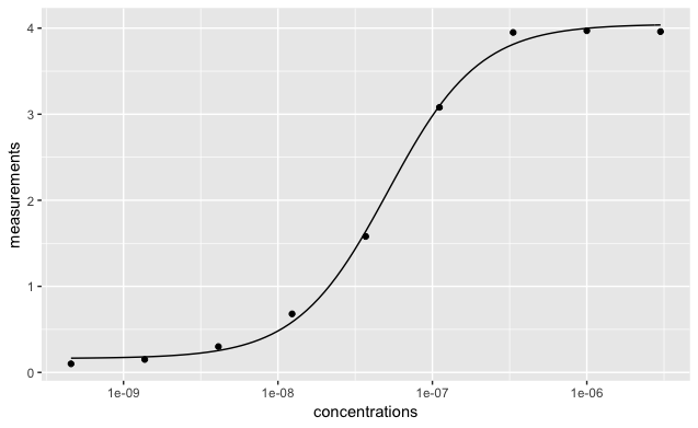
Using the standards for new samples
In my case I was just after Kd (Mid) values but if you wanted to now use this standard curve to return a concentration from a measurement then you can rearrange the formula and use the parameters calculated with nls above.
CalcConc <- function(Background, Mid, Slope, Bmax, y) {
  as.numeric(Mid * ((Background - Bmax)/(y - Bmax) - 1)^(1/Slope))
}


CalcConc( coef(fit)["Background"],
          coef(fit)["Mid"],
          coef(fit)["Slope"],
          coef(fit)["Bmax"],
          y = 3.5 )

#[1] 5.516211e-08
And we’re done!